tynbl.github.io
实战案例5-1:根据海报预测电影分类
- 项目:根据可穿戴设备识别用户行为
- 作者:梁斌
- 日期:2017/10
- 提问:小象问答
- 声明:小象学院拥有完全知识产权的权利;只限于善意学习者在本课程使用,不得在课程范围外向任何第三方散播。任何其他人或机构不得盗版、复制、仿造其中的创意,我们将保留一切通过法律手段追究违反者的权利
1. 项目描述:
电影海报是获取电影内容和类型的途径之一。用户可以通过海报的一些信息(如:颜色,演员的表情等)推测出其所属的类型(恐怖片,喜剧,动画等)。研究表明图像的颜色是影响人类感觉(心情)的因素之一,在本次项目中,我们会通过海报的颜色信息构建模型,并对其所属的电影类型进行推测。
2. 数据集描述:
- Kaggle提供的数据集。数据采集自IMDB网站,包含电影信息(MovieGenre.csv)和电影的海报图片(SampleMoviePosters)。
MovieGenre.csv 数据字典:
- imdbId,IMDB中电影的Id
- Imdb Link,IMDB中电影的链接
- Title,电影名称
- IMDB Score,IMDB中电影的评分
- Genre,电影类型
- Poster,电影海报链接
SampleMoviePosters 目录中包含了电影的海报图片(*.jpg),图片的文件名为IMDB中对应的电影Id
3. 项目任务:
- 3.1 数据查看及处理
- 3.2 特征表示
- 3.3 数据建模及验证
- 3.4 数据预测
4. 项目实现:
# 引入必要的包
import csv
import os
import numpy as np
import pandas as pd
import matplotlib.pyplot as plt
import seaborn as sns
import time

%matplotlib inline
# 解决matplotlib显示中文问题
# 仅适用于Windows
plt.rcParams['font.sans-serif'] = ['SimHei']  # 指定默认字体
plt.rcParams['axes.unicode_minus'] = False  # 解决保存图像是负号'-'显示为方块的问题

# MacOS请参考 http://wenda.chinahadoop.cn/question/5304 修改字体配置
4.1 数据查看及处理
# 指定数据集路径
dataset_path = '../data'
csv_filepath = os.path.join(dataset_path, 'MovieGenre.csv')
poster_path = os.path.join(dataset_path, 'SampleMoviePosters')

# 加载数据
movie_df = pd.read_csv(csv_filepath, encoding='ISO-8859-1',
                       usecols=['imdbId', 'Title', 'IMDB Score', 'Genre'])
movie_df.head()
| imdbId | Title | IMDB Score | Genre | |
|---|---|---|---|---|
| 0 | 114709 | Toy Story (1995) | 8.3 | Animation|Adventure|Comedy |
| 1 | 113497 | Jumanji (1995) | 6.9 | Action|Adventure|Family |
| 2 | 113228 | Grumpier Old Men (1995) | 6.6 | Comedy|Romance |
| 3 | 114885 | Waiting to Exhale (1995) | 5.7 | Comedy|Drama|Romance |
| 4 | 113041 | Father of the Bride Part II (1995) | 5.9 | Comedy|Family|Romance |
# 处理genre列,使其只包含一种类型
movie_df['Single Genre'] = movie_df['Genre'].str.split('|', expand=True)[0]
print('csv有{}条记录。'.format(len(movie_df)))
movie_df.head()
csv有40108条记录。
| imdbId | Title | IMDB Score | Genre | Single Genre | |
|---|---|---|---|---|---|
| 0 | 114709 | Toy Story (1995) | 8.3 | Animation|Adventure|Comedy | Animation |
| 1 | 113497 | Jumanji (1995) | 6.9 | Action|Adventure|Family | Action |
| 2 | 113228 | Grumpier Old Men (1995) | 6.6 | Comedy|Romance | Comedy |
| 3 | 114885 | Waiting to Exhale (1995) | 5.7 | Comedy|Drama|Romance | Comedy |
| 4 | 113041 | Father of the Bride Part II (1995) | 5.9 | Comedy|Family|Romance | Comedy |
# 将海报文件路径和csv进行合并操作
# 构造海报dataframe
poster_df = pd.DataFrame(columns=['imdbId', 'img_path'])

poster_df['img_path'] = os.listdir(poster_path)
poster_df['imdbId'] = poster_df['img_path'].str[:-4].astype('int')

poster_df.head()
| imdbId | img_path | |
|---|---|---|
| 0 | 10040 | 10040.jpg |
| 1 | 10057 | 10057.jpg |
| 2 | 10071 | 10071.jpg |
| 3 | 10155 | 10155.jpg |
| 4 | 10195 | 10195.jpg |
data_df = movie_df.merge(poster_df, on='imdbId', how='inner')
data_df.drop_duplicates(subset=['imdbId'], inplace=True)
print('数据集有{}条记录。'.format(len(data_df)))
data_df.head()
训练集有998条记录。
| imdbId | Title | IMDB Score | Genre | Single Genre | img_path | |
|---|---|---|---|---|---|---|
| 0 | 24252 | Liebelei (1933) | 7.7 | Drama|Romance | Drama | 24252.jpg |
| 1 | 25316 | It Happened One Night (1934) | 8.2 | Comedy|Romance | Comedy | 25316.jpg |
| 2 | 25164 | The Gay Divorcee (1934) | 7.6 | Comedy|Musical|Romance | Comedy | 25164.jpg |
| 3 | 17350 | The Scarlet Letter (1926) | 7.8 | Drama | Drama | 17350.jpg |
| 4 | 25586 | Of Human Bondage (1934) | 7.3 | Drama|Romance | Drama | 25586.jpg |
# 查看各电影类型的数量
data_df.groupby('Single Genre').size().sort_values(ascending=False)
Single Genre
Drama          354
Comedy         266
Crime           84
Short           63
Adventure       53
Action          37
Animation       23
Biography       20
Documentary     17
Romance         16
Fantasy         12
Horror          12
Mystery         12
Western         11
Musical          8
Family           3
War              3
History          2
Music            2
dtype: int64
# 可视化各类别的数量统计图
plt.figure()

# 训练集
sns.countplot(x='Single Genre', data=data_df)

plt.title('电影类型数量统统计')
plt.xticks(rotation='vertical')
plt.xlabel('电影类型')
plt.ylabel('数量')

plt.tight_layout()
<IPython.core.display.Javascript object>

有些电影类型过于少,不利于预测。将上述问题抓换为3分类问题:Drama, Comedy, Other
cond = (data_df['Single Genre'] != 'Drama') & (data_df['Single Genre'] != 'Comedy')
data_df.loc[cond, 'Single Genre'] = 'Other'
data_df.reset_index(inplace=True)
# 查看各电影类型的数量
data_df.groupby('Single Genre').size().sort_values(ascending=False)
Single Genre
Other     378
Drama     354
Comedy    266
dtype: int64
4.2 特征表示
from skimage import io, exposure

# 提取出每个图片的直方图作为颜色特征
def extract_hist_feat(img_path, nbins=50, as_grey=True):
    """
        提取出每个图片的直方图作为颜色特征
        img_path: 图片路径
        nbins: 直方图bin的个数,即特征的维度
    """
    image_data = io.imread(img_path, as_grey=as_grey)
    # 直方图均衡化
    eq_image_data = exposure.equalize_hist(image_data)

    if as_grey:
        # 灰度图片
        # 提取直方图特征
        hist_feat, _ = exposure.histogram(eq_image_data, nbins=nbins)
    else:
        # 彩色图片
        # 每个通道提取直方图,然后做合并
        # 学员自行完成
        # 提示:获取每个通道上的图像数据,然后分别做直方图统计
        # 假设,每个通道得到50维的向量,最后的彩色直方图向量维度为 50 x 3
        pass

    # 统计直方图频率(归一化特征),避免因为图片的尺寸不同导致直方图统计个数的不同,
    norm_hist_feat = hist_feat / sum(hist_feat)
    return norm_hist_feat
# 测试一张图片
img_path = os.path.join(poster_path, data_df.loc[1, 'img_path'])
hist_feat = extract_hist_feat(img_path)
print(hist_feat)
[ 0.02417172  0.01929227  0.01757012  0.01572495  0.01689355  0.01935378
  0.02128096  0.01806216  0.0195383   0.0239667   0.02121945  0.02007135
  0.02144497  0.02228555  0.02089142  0.02021486  0.02105544  0.01896424
  0.01962031  0.02035837  0.01945629  0.0206864   0.01935378  0.02123995
  0.01939478  0.02095293  0.01988683  0.01978432  0.02005084  0.01992783
  0.01982532  0.01970231  0.01974332  0.01978432  0.01988683  0.01968181
  0.01964081  0.01945629  0.02003034  0.01923077  0.01962031  0.02000984
  0.02017386  0.0195178   0.02005084  0.01968181  0.01990733  0.02082992
  0.01986633  0.0206454 ]
data_df.index
RangeIndex(start=0, stop=998, step=1)
# 对数据集中的每张图片进行特征提取
n_feat_dim = 100
n_samples = len(data_df)

# 初始化特征矩阵
X = np.zeros((n_samples, n_feat_dim))
print(X.shape)

for i, r_data in data_df.iterrows():
    if (i + 1) % 100 == 0:
        print('正在提取特征,已完成{}个海报'.format(i + 1))
    img_path = os.path.join(poster_path, r_data['img_path'])
    hist_feat = extract_hist_feat(img_path, n_feat_dim)
    # 赋值到特征矩阵中
    X[i, :] = hist_feat.copy()

# 可以尝试对特征进行归一化处理
(998, 100)
正在提取特征,已完成100个海报
正在提取特征,已完成200个海报
正在提取特征,已完成300个海报
正在提取特征,已完成400个海报
正在提取特征,已完成500个海报
正在提取特征,已完成600个海报
正在提取特征,已完成700个海报
正在提取特征,已完成800个海报
正在提取特征,已完成900个海报
# 获取标签名称
target_names = data_df['Single Genre'].values

from sklearn.preprocessing import LabelEncoder
label_enc = LabelEncoder()
y = label_enc.fit_transform(target_names)
print('电影类型:', label_enc.classes_)
print('y:', y)
电影类型: ['Comedy' 'Drama' 'Other']
y: [1 0 0 1 1 1 0 2 2 1 1 1 1 1 1 1 2 2 2 2 0 1 0 0 2 1 2 0 0 2 2 1 2 1 2 2 2
 1 1 2 2 1 1 0 2 0 0 0 0 2 0 2 1 0 0 2 0 0 2 0 2 2 2 1 0 1 2 2 1 1 2 1 1 0
 0 1 2 2 2 1 2 2 2 1 0 2 1 2 1 0 0 0 0 1 0 1 2 2 0 0 2 2 1 2 1 2 2 0 2 0 2
 0 0 2 2 1 2 1 2 2 0 2 2 1 1 2 2 2 1 1 2 2 2 1 2 1 0 2 1 0 1 2 1 1 1 1 2 0
 2 1 1 1 2 1 2 2 0 1 0 2 0 0 2 0 2 2 2 0 2 1 0 2 0 2 0 0 2 1 2 0 2 2 1 2 2
 2 0 1 2 1 0 1 0 0 0 1 2 1 1 1 1 0 0 1 0 1 1 0 0 1 2 2 1 1 2 1 1 1 2 1 2 2
 2 0 2 1 1 1 0 0 0 1 1 1 0 1 0 1 1 2 2 2 0 2 0 2 0 1 0 1 2 1 0 0 1 1 2 1 0
 2 2 1 2 0 2 2 1 1 2 0 2 0 2 0 2 0 2 1 2 2 2 1 0 2 2 2 1 1 2 0 2 1 2 2 2 1
 0 0 1 2 0 2 2 0 0 0 0 2 0 2 0 2 0 0 1 2 2 0 1 1 2 0 0 2 2 2 0 0 0 2 1 2 2
 0 2 1 2 2 2 1 2 0 2 1 2 1 2 0 2 1 0 1 0 2 0 1 1 1 2 1 2 0 0 0 1 0 1 1 1 2
 1 0 2 2 0 0 1 2 2 2 1 2 0 0 2 1 2 2 0 1 1 0 1 1 1 1 0 0 0 0 1 1 1 0 1 0 2
 0 1 0 2 1 2 0 2 1 1 0 0 0 2 1 0 0 1 2 2 1 0 0 1 1 2 2 2 0 2 2 1 0 2 2 2 2
 2 2 0 1 2 2 2 0 2 2 2 0 2 2 2 1 1 1 1 1 1 2 1 2 1 2 2 2 2 1 1 0 1 1 2 2 2
 0 1 1 1 1 1 2 1 0 2 1 0 0 2 1 1 1 2 2 1 1 1 1 1 2 2 1 2 1 0 1 0 1 1 0 1 0
 1 1 1 1 2 1 1 1 2 1 2 1 1 0 1 2 0 1 2 0 2 0 0 0 2 2 1 1 1 0 1 2 1 2 2 0 2
 1 2 1 0 0 1 1 0 0 2 0 2 0 0 0 0 2 2 1 1 1 1 1 2 2 1 2 1 0 2 1 0 0 0 2 2 2
 0 1 1 1 1 1 2 1 0 0 0 1 2 1 1 2 1 2 2 0 0 2 0 2 2 2 0 2 2 2 2 1 0 2 1 2 1
 2 2 0 2 1 1 1 1 2 0 0 0 0 2 1 1 0 1 2 1 1 0 1 2 0 0 1 0 0 1 2 1 1 0 1 2 1
 2 0 1 1 1 1 1 2 1 1 1 2 1 2 2 0 1 1 2 1 0 0 2 0 1 0 2 2 2 1 1 2 2 2 2 2 0
 0 2 2 1 2 2 1 1 0 2 0 0 1 1 1 1 2 1 1 0 1 0 2 0 2 0 2 1 1 2 2 1 0 0 1 2 2
 2 1 0 0 2 2 1 0 1 0 2 1 0 1 1 0 0 2 0 1 1 0 0 0 0 1 0 0 2 0 0 2 0 1 2 0 1
 2 2 2 1 2 1 1 0 1 0 2 1 2 1 1 0 1 2 1 0 1 2 1 1 1 2 0 2 2 0 1 1 1 1 2 2 2
 2 2 1 2 2 2 2 1 2 1 0 2 1 2 2 1 1 0 0 1 2 0 2 1 2 2 1 1 1 1 2 2 1 0 0 2 1
 1 1 0 0 1 2 1 0 2 1 2 1 1 1 2 1 2 0 2 1 0 2 0 2 2 2 0 2 0 2 0 2 2 2 2 2 2
 2 2 1 1 1 2 0 0 1 1 1 2 1 1 2 0 0 2 2 2 2 2 0 1 0 2 0 2 0 0 0 1 1 2 1 1 1
 1 2 2 2 2 2 2 2 1 1 2 0 0 1 1 1 1 0 0 0 0 1 0 0 1 2 2 2 2 0 1 1 0 0 1 1 2
 1 2 2 2 1 0 1 2 2 0 2 2 1 2 2 1 1 2 2 1 2 2 1 2 1 2 0 2 2 1 2 2 2 0 1 1]
# 分割训练集和测试集
from sklearn.model_selection import train_test_split

X_train, X_test, y_train, y_test = train_test_split(X, y, test_size=1/4, random_state=0)
print('训练集样本数:', len(X_train))
print('测试集样本数:', len(X_test))
训练集样本数: 748
测试集样本数: 250
至此,数据集已经处理完毕,接下来可以进行数据建模了。
4.3 数据建模及验证
from sklearn.model_selection import GridSearchCV

def train_model(X_train, y_train, X_test, y_test, model_config, cv_val=3):
    """
        返回对应的最优分类器及在测试集上的准确率
    """
    model = model_config[0]
    parameters = model_config[1]

    if parameters is not None:
        # 需要调参的模型
        clf = GridSearchCV(model, parameters, cv=cv_val, scoring='accuracy')
        clf.fit(X_train, y_train)
        print('最优参数:', clf.best_params_)
        print('验证集最高得分: {:.3f}'.format(clf.best_score_))
    else:
        # 不需要调参的模型,如朴素贝叶斯
        model.fit(X_train, y_train)
        clf = model

    test_acc = clf.score(X_test, y_test)
    print('测试集准确率:{:.3f}'.format(test_acc))
    return clf, test_acc
from sklearn.neighbors import KNeighborsClassifier
from sklearn.linear_model import LogisticRegression
from sklearn.svm import SVC
from sklearn.tree import DecisionTreeClassifier
from sklearn.naive_bayes import GaussianNB
from sklearn.ensemble import RandomForestClassifier
from sklearn.ensemble import GradientBoostingClassifier

model_dict = {'kNN':    (KNeighborsClassifier(),        {'n_neighbors': [5, 10, 15]}),
              'LR':     (LogisticRegression(),          {'C': [0.01, 1, 100]}),
              'SVM':    (SVC(),                         {'C': [100, 1000, 10000]}),
              'DT':     (DecisionTreeClassifier(),      {'max_depth': [50, 100, 150]}),
              'GNB':    (GaussianNB(), None),
              'RF':     (RandomForestClassifier(),      {'n_estimators': [100, 150, 200]}),
              'GBDT':   (GradientBoostingClassifier(),  {'learning_rate': [0.1, 1, 10]})}
results_df = pd.DataFrame(columns=['Accuracy (%)'], index=list(model_dict.keys()))
results_df.index.name = 'Model'
models = []

for model_name, model_config in model_dict.items():
    print('训练模型:', model_name)
    model, acc = train_model(X_train, y_train,
                          X_test, y_test,
                          model_config)
    models.append(model)
    results_df.loc[model_name] = acc * 100
    print()
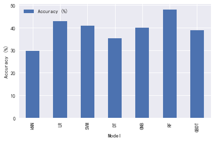
训练模型: kNN
最优参数: {'n_neighbors': 15}
验证集最高得分: 0.366
测试集准确率:0.296

训练模型: LR
最优参数: {'C': 100}
验证集最高得分: 0.382
测试集准确率:0.428

训练模型: SVM
最优参数: {'C': 10000}
验证集最高得分: 0.381
测试集准确率:0.408

训练模型: DT
最优参数: {'max_depth': 100}
验证集最高得分: 0.368
测试集准确率:0.352

训练模型: GNB
测试集准确率:0.400

训练模型: RF
最优参数: {'n_estimators': 200}
验证集最高得分: 0.402
测试集准确率:0.480

训练模型: GBDT
最优参数: {'learning_rate': 1}
验证集最高得分: 0.352
测试集准确率:0.388
# 保存结果
results_df.to_csv('./pred_results.csv')

results_df.plot(kind='bar')
plt.ylabel('Accuracy (%)')
plt.tight_layout()
plt.savefig('./pred_results.png')
plt.show()
# 保存最优模型
import pickle

best_model_idx = results_df.reset_index()['Accuracy (%)'].argmax()
best_model = models[best_model_idx]

saved_model_path = './predictor.pkl'
with open(saved_model_path, 'wb') as f:
    pickle.dump(best_model, f)
4.4 数据预测
# 加载保存的模型
with open(saved_model_path, 'rb') as f:
predictor = pickle.load(f)
# 进行预测
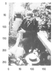
imdb_id = 2544
img_path = os.path.join(poster_path, str(imdb_id) + '.jpg')
poster_feat = extract_hist_feat(img_path, n_feat_dim)
pred_result = predictor.predict(poster_feat.reshape(1, -1))
pred_genre = label_enc.inverse_transform(pred_result)
print('预测类型:', pred_genre)
true_genre = data_df[data_df['imdbId'] == imdb_id ]['Single Genre'].values
print('实际类型:', true_genre)
plt.figure()
plt.grid(False)
plt.imshow(io.imread(img_path))
预测类型: ['Drama']
实际类型: ['Drama']


<matplotlib.image.AxesImage at 0x20530452be0>
5. 项目总结
- 该项目实现了一个可以根据海报预测电影分类的项目,包括:
- 图像数据处理及操作
- 数据可视化
- 数据集特征、标签的处理
- 模型的持久化
- 课后学员可模仿该项目的流程与操作,在现有数据集上通过完成以下任务,观察对模型的性能有何影响
- 使用RGB三个通道上的直返图特征
- 使用特征归一化
- 调整适当的超参数范围,优化模型
- 该项目有配套的Python代码